Market Making and Mean Reversion
Switching gears from AI programming for a bit, it seems that you can make good amounts of money by betting on mean-reverting instruments? A paper by Chakraborty and Kearns shows that market making strategies can be consistently profitable on financial instruments that tend to bounce back to their average price. Their math proves that as long as there’s sufficient price volatility around a stable mean, profits should grow linearly with time.
What makes this particularly surprising to me is that the mathematics suggests this isn’t just a temporary inefficiency, but a structural feature of mean-reverting markets that could theoretically generate consistent profits over time. The key theoretical finding is that for a financial instrument (commodities, forex etc.), if \(K\) represents price volatility (sum of absolute price movements) and \(z\) is the net price change, profit equals \((K-z²)/2\). For mean-reverting processes, \(E[K]\) grows linearly with time while \(E[z²]\) remains bounded by a constant, creating increasing expected profits over longer time horizons. Accumulated volatility (\(K\)) sums up every little price wiggle, while the final spread (\(z\)) just captures the net difference from start to finish. With mean reversion, prices may dance wildly but always come back close to the average, so despite lots of movement, the overall drift remains small. For a retail investor, this means that even if the end result seems modest, there were plenty of opportunities to capture gains along the way.
The market making strategy in the paper requires placing and adjusting orders after virtually every price change - something practically impossible for retail investors without specialized systems. On the other hand, pairs trading, while definitely complex, at least operates on timeframes and mechanisms available to dedicated retail traders. Pairs trading is another strategy that also exploits mean reversion, and unlike market making, which profits from price oscillations while maintaining neutral exposure, pairs trading involves taking specific directional positions based on the relationship between two correlated securities.
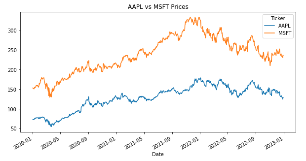
Let’s take AAPL and MSFT for example. This the stock price movement for both between 2020 to 2023, and you can see they generally move together but sometimes diverge significantly.:

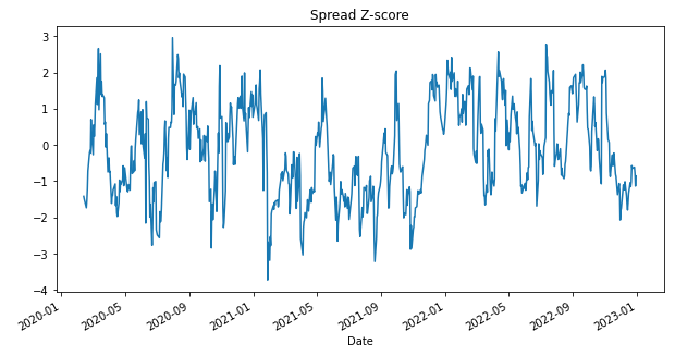
After calculating the ‘spread’ (AAPL minus MSFT price) and normalizing it using z-scores, we get the following z-spread:

This z-score simply tells us how unusual the current spread is compared to its recent history - specifically, how many standard deviations it sits from its 30-day moving average. The bottom chart reveals the pattern we’re looking for: the z-score oscillates between extremes but consistently reverts to the mean. When the z-score exceeds +1.5 (spread is unusually wide), it suggests shorting AAPL and buying MSFT. When it drops below -1.5 (spread is unusually narrow), the opposite trade makes sense.
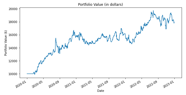
If we execute this simple strategy, we nearly double our portfolio in 3 years. That’s a CAGR of ~20%!

You can follow along with the code here:
import pandas as pd
import numpy as np
import yfinance as yf
import matplotlib.pyplot as plt

tickers = ['AAPL', 'MSFT']
# Download adjusted close prices for a chosen period
data = yf.download(tickers, start='2020-01-01', end='2023-01-01')['Close']
data.dropna(inplace=True)

data.plot(figsize=(10,5), title="AAPL vs MSFT Prices")
plt.show()

spread = data['AAPL'] - data['MSFT']
# Compute rolling z-score of the spread
window = 30
spread_mean = spread.rolling(window).mean()
spread_std = spread.rolling(window).std()
spread_z = (spread - spread_mean) / spread_std

spread_z.plot(figsize=(10,5), title="Spread Z-score")
plt.show()

entry_threshold = 1.5
signals = pd.DataFrame(index=spread_z.index, columns=['position'])
signals['position'] = 0

# Signal definitions: +1 means long AAPL, short MSFT; -1 means short AAPL, long MSFT.
signals.loc[spread_z < -entry_threshold, 'position'] = 1
signals.loc[spread_z > entry_threshold, 'position'] = -1

# Carry forward positions until an exit signal (spread_z crosses 0)
signals['position'] = signals['position'].replace(to_replace=0, method='ffill')

# Calculate daily returns
returns = data.pct_change()

# Compute strategy returns: if long (position=1) profit = (AAPL return - MSFT return); if short, reverse.
strategy_returns = signals['position'].shift(1) * (returns['AAPL'] - returns['MSFT'])

# Compute cumulative returns
cumulative_returns = (1 + strategy_returns.fillna(0)).cumprod() - 1

cumulative_returns.plot(figsize=(10,5), title="Cumulative Strategy Returns")
plt.show()

initial_capital = 10000
# Convert cumulative returns to portfolio values (initial capital * (1 + return))
portfolio_value = initial_capital * (1 + cumulative_returns)
portfolio_value.plot(figsize=(10,5), title="Portfolio Value (in dollars)")
plt.ylabel("Portfolio Value ($)")
plt.show()
This is a vanilla implementation and reality will be far messier. Transaction costs can significantly impact returns, especially if you’re making frequent trades. Market impact can also be a factor - if you’re trading large positions, your own trades might move the market against you. Tax considerations can substantially affect net returns. Most importantly, the mean-reverting relationship between securities can break down, particularly during market stress or when fundamental changes occur in one of the companies. The strategy implicitly assumes that past statistical relationships will continue into the future, which isn’t always the case. But something worth thinking about.
As a retail investor, I’ve typically focused only on where stocks end up rather than their journey. But the math here (\(E[K]\) growing linearly while \(E[z²]\) remains bounded) suggests I’m leaving money on the table. These volatility patterns contain substantial profit opportunity that traditional buy-and-hold approaches simply ignore.